On Tide and Terrain

The county is not the country

An election may turn on the price of groceries, the performance of a president, a war, or a candidate’s ability to hold together an uneasy coalition. That is the national account of an election, and it is indispensable. But the national account does not explain why a county changes more than the state around it or why a neighboring county barely changes at all.

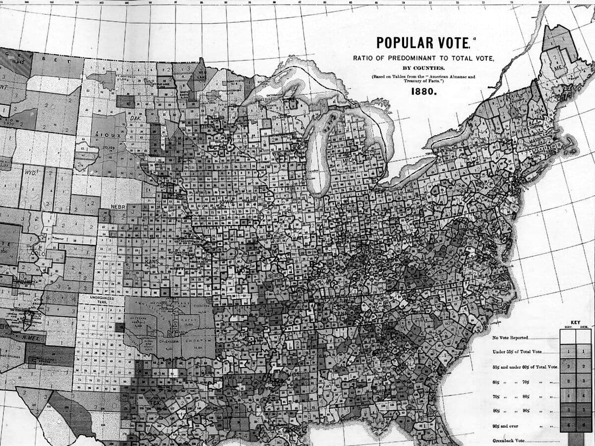
Two counties in the same state can respond very differently to the same presidential election. One may shift sharply from its previous result while the other barely moves. That difference is clear once the votes are counted. Could anything known before Election Day have helped us anticipate it?

This is the question behind Providence Strategy’s original research question. We are not attempting to replace polling with a map, nor to claim that county-level statistics reveal what any individual voter thinks. Polls describe opinion at a point in time, while county returns record how people voted, in aggregate, after the fact. They measure different things. The public polling record also resists caricature: after important errors in 2016 and 2020, the American Association for Public Opinion Research judged the public polls of 2024 comparatively accurate. [12]

Our point of departure is narrower. We want to distinguish the movement common to a state from the movement peculiar to its counties. We call the first the tide and the second the terrain. The metaphor is useful as long as it does not decide the conclusion in advance. A coastline can change; so can a county’s electorate. What matters is whether we can measure the difference and whether our measurements carry information into the next election.

Why begin with economics?

We began with a straightforward possibility: voters in places losing jobs, residents, or purchasing power might turn against the president’s party. If that pattern held across elections, local economic data could help us identify where support was likely to shift.

The question has a long history in economics and political science. Voters may judge the economy through their own finances, their view of national conditions, or both. D. Roderick Kiewiet’s work distinguished personal experience from judgments about national unemployment and inflation. Daniel Hopkins has since described how American political behavior has become increasingly nationalized. Neither argument implies that a county’s economic condition must translate mechanically into a county’s vote. [8, 9]

More importantly, the empirical literature does not speak with one voice. Research by de Benedictis-Kessner and Warshaw found evidence that the president’s party is held accountable for local economic performance across several levels of American government. Autor, Dorn, Hanson, and Majlesi identified political realignment in areas exposed to Chinese import competition. These studies provide evidence that local economic conditions can matter at the ballot box. Any account that dismisses those conditions altogether would have to explain their findings. [10, 11]

Other research raises questions about how consistently voters hold incumbents responsible for local economic performance. In a 2026 study, B. K. Song tested 144 plausible specifications across several types of elections. Among the presidential specifications, 61 percent showed a positive, statistically significant relationship. The finding did not hold across the full set, and results for several other offices were less consistent still. That does not rule out local economic voting, but it shows how much the conclusion can depend on the measures and methods used. [13]

The useful question for our research is therefore not whether economics affects politics in some abstract sense. It is whether the local economic indicators available in our county panel add reliable information about where a presidential result will diverge from statewide movement. That is a prediction question as well as an explanation question, and the two must be evaluated separately.

The measurement: movement after the tide

We begin with the Democratic share of the two-party presidential vote in each county. County swing is the change in that share between consecutive presidential elections. State swing is the corresponding change for the state. Relative swing subtracts the second from the first. A positive result indicates that a county moved more Democratic—or less Republican—than its state. A negative result means the county moved more Republican—or less Democratic—than its state.

The absolute value of relative swing removes the direction. It tells us how far a county departed from the statewide movement. This is our primary historical measure of electoral volatility. A county can remain safely Republican or safely Democratic and still be volatile by this definition. A closely divided county, meanwhile, may barely change between elections. How close the race is, which party gains, and how far the county moves relative to its state are three different questions.

For example, suppose a county’s Democratic two-party share rises four percentage points while its state rises three. The county’s relative swing is +1 percentage point; the magnitude of its departure is 1 point. If the county instead falls two points while the state rises three, its relative swing is −5 points and its departure magnitude is 5. Neither departure magnitude tells us whether the county is competitive or consequential in the Electoral College.

The exploratory study follows county results across seven presidential elections, from 2000 through 2024. Those elections give us six transitions to examine, with 18,097 eligible observations across 3,096 county units. The study excludes Alaska because its presidential returns are reported using election districts that are not consistently equivalent to counties; it also applies outcome and geographic-continuity exclusions. The research inventory includes 231 socioeconomic features constructed for the analysis, 14 features describing political history, and several definitions of the outcome being measured. These counts apply to this exploratory study. They should not be read as a count of all U.S. counties or as the specifications of a released production dataset. [P1]

County presidential returns can be sourced from the MIT Election Data and Science Lab and compared with the federal results that the Federal Election Commission compiles from state election offices. Demographic and economic context comes from the Census Bureau, Bureau of Labor Statistics, Bureau of Economic Analysis, and Internal Revenue Service, among other public programs. Each source uses its own definitions and publication schedule, and the sources differ in how they revise estimates and which geographic areas they cover. Those differences need to be accounted for when combining the data. [1–7]

That last point is decisive for forecasting. An economic estimate describing conditions before an election may have been published or revised only afterward. A model trained using such a number is suitable for retrospective research, but it has not demonstrated that it could have made the same prediction in real time. The research inventory records which information was available before Election Day and separately identifies revised estimates and measurements treated as structurally fixed. A credible P.Vol forecast needs to retain those distinctions and establish what was actually known at the forecast date. [P1]

What the first tests actually suggest

The first result is that the history and composition of a county contain substantially more information about its relative electoral movement than the recent economic changes examined here. In the exploratory study, political history and slow-moving structural indicators explained about 51 percent of within-state, within-election variation in relative swing in the fitted sample. Including changes in population and migration increased the fitted R-squared by about 0.4 percentage points. Labor-market changes added roughly 0.5–1.2 points, depending on the period and available data; other economic variables added around 0.3–0.4 points. These figures measure gains in explanatory power, not changes in vote share. Because the estimates came from different samples, they cannot simply be added together. [P1]

The second finding concerns whether local economic conditions help explain losses for the president’s party. That party lost national two-party vote share in five of the six election transitions studied, from 2000–2004 through 2020–2024. But none of the ten claims tested about local economic conditions and incumbent-party performance met the project’s standard for a consistently robust relationship across elections and model specifications. The conclusion is limited: the indicators tested did not reliably identify where the incumbent party would lose more ground than it did statewide. [P1]

The third result concerns the size of a move rather than its partisan direction. In the exploratory regressions, larger state-relative departures were associated with smaller electorates, lower educational attainment, greater reliance on government-transfer income, and a history of larger relative swings. Additional associations appeared for population relative to its earlier peak and for unusual population growth or decline relative to the state. These patterns were not identical in every test. Nor should they be interpreted as the preferences or motives of the individuals living in those places. [P1]

One nuance matters. Population growing much faster than a state—and population shrinking much faster—can each accompany greater departure magnitude. This is not simply a theory of hardship. A fast-growing suburb may be changing politically even while its economy is healthy. Differences between counties do not, by themselves, show what will happen when conditions change within a particular county. A characteristic associated with greater volatility across counties may not cause more volatility when it changes in one place. The project’s county fixed-effect exercises generally found little evidence of such a within-county effect. [P1]

These findings push us away from the original idea of a political-distress index. They do not push us away from prediction. If some counties have durable characteristics associated with unusually large moves, we can test whether those characteristics help rank future risk. That is a more demanding claim than describing correlations. It is also a more useful one.

A modest but measurable forecasting signal

A model that fits the past may know very little about the future. County-level election data make this especially easy to forget. Thousands of geographic observations do not supply thousands of independent national elections. For the period examined here, there are six transitions and only a handful of genuinely distinct political environments. A model can mistake the peculiar character of 2016 for a permanent law.

The project’s exploratory validation addresses that problem by holding out whole elections. In its large-move classification exercise, models using political history and structural information achieved area-under-the-curve (AUC) scores of approximately 0.61–0.75 on selected held-out elections for identifying counties in the top decile of relative departure. An AUC of 0.5 corresponds to no ranking discrimination; an AUC of 1 would represent perfect separation. The stronger exploratory configurations also achieved approximately twofold lift among the counties placed in the highest predicted-risk decile: their concentration of realized large movers was roughly double a random selection. These are results from an unpublished research pipeline, not audited public forecasts. [P1]

This is the piece of evidence on which the ambition for P.Vol can reasonably rest. It suggests that a county-ranking model may extract some useful signal from what is known beforehand. It does not establish reliable probabilities, precise vote-share forecasts, or equally strong performance in every election.

Indeed, the same study reported little Brier-score improvement over baseline event probabilities and substantial overconfidence in parts of its probability forecasts. A separate project cross-check, using a different county-margin target, sample, and shorter training windows, found weaker out-of-sample rank correlations for departure magnitude—roughly 0.03 to 0.24. Its linear models gained only about 0.03–0.04 in rank correlation from additional population and economic inputs, and some boosted-model improvements were statistically uncertain. These results cannot be combined numerically with the first study’s AUC estimates. But they point toward the same constraint: useful ranking is possible in some settings; strong and stable prediction remains unproven. [P1, P2]

Even the scale of volatility changes sharply by election. In the exploratory panel, the proportion of counties moving more than five percentage points relative to their states varied from less than 1 percent in 2024 to nearly 45 percent in 2016. A five-point threshold does not mean the same thing in every political environment. We therefore distinguish a raw departure measured in percentage points from a county’s relative position in the distribution for that election. A forecast of which counties will rank as unusually volatile is not yet a forecast of how many points each will move. [P1]

This is why P.Vol should begin as a relative risk tier. We can say that the available evidence puts a county among the places most exposed to an unusually large departure under a specified model. Until calibration is demonstrated, we should not convert that tier into a claim such as “this county has a 70 percent chance of swinging sharply.” A percentile is a ranking. It is not a probability.

Building P.Vol without pretending to know more than we do

The historical measure is straightforward: for each election, calculate the magnitude of each county’s relative swing and rank it against a defined, eligible set of counties. That yields realized P.Vol—the unusualness of a county’s movement in an election already held. Expected P.Vol is harder. It must be estimated before the election from information that would actually have been available at the chosen forecast date.

The first forecast should use a deliberately modest set of predictors: previous relative swings, the size of the electorate, historical volatility, demographic structure, population trajectory, and a limited group of economic indicators whose data vintage can be verified. We should test simpler models before introducing elaborate composites. Variables belong in the model because they improve performance on elections not used to select them, not because they produce an intuitively appealing story about a place.

We propose the following discipline. Before scoring an election, publish the county universe, outcome definition, feature list, release cutoffs, model version, uncertainty method, and benchmark forecasts. Train only on earlier election cycles. Evaluate on each subsequent election without using that election to revise the model. Report results separately by election so an average does not conceal a failure in an important cycle. Compare performance with basic alternatives: previous relative swing, historical volatility, electorate size, and an uninformative ranking. [P1]

Evaluation should answer practical questions rather than only statistical ones. Among the counties ranked in the highest risk tier, what fraction actually landed among the largest movers? Was that capture rate materially better than a baseline? Did the ordering hold in both low-volatility and high-volatility elections? How different were the results for small and large electorates? How stable were the rankings when county boundaries, economic vintages, or model choices changed? And if a calibrated probability is eventually published, did events occur about as frequently as predicted?

There is a structural difficulty in a nationwide county model: counties do not move independently. Neighboring places can respond to the same political and cultural developments. The exploratory work found substantial spatial correlation in relative swings. Validation must therefore avoid treating thousands of adjacent observations as independent confirmation of a national result. It must preserve election holdouts and use uncertainty estimates that respect geographic dependence. [P1]

A further caution concerns the meaning of our outcome. The state’s observed swing is useful for a retrospective decomposition because it lets us ask which counties diverged from the statewide result. Before the election, however, that state swing is unknown. To forecast a county’s eventual result, an analyst must separately forecast the state and the county’s position relative to it. A future polling-adjusted system should keep those components separate, including the uncertainty attached to each. It should never relabel a statewide polling miss as county-specific volatility.

Volatility is not electoral consequence

The places most likely to move are not necessarily the places most likely to decide an election. A county with a few thousand votes can experience an exceptional relative swing while making little difference to the statewide total. A large county can make a substantial contribution to the statewide margin after a comparatively ordinary change in vote share. Neither fact is a contradiction.

Providence Intelligence should therefore keep two questions distinct. P.Vol addresses the likelihood or relative risk of unusual county movement. Electoral consequence asks what a movement of a given size and direction would mean for the votes that determine a state, and ultimately for the Electoral College. The second requires turnout, electorate size, statewide competitiveness, correlated movement across counties, and a clearly stated election scenario. A model that answers one question cannot be assumed to answer the other.

This distinction is practical. An analyst studying emerging political coalitions may care deeply about a small county whose direction of travel departs from its neighbors. An analyst studying the path to 270 electoral votes may care more about a populous suburban county in a narrowly contested state. Both observations can be true; they belong on different axes of an intelligence product.

What the research cannot yet establish

The county is an informative unit of analysis, but it is not an individual voter. County patterns cannot tell us whether particular residents changed their minds, whether different groups turned out, or whether migration changed who lived there. Even a reliable county-level association is not a causal explanation.

The historical sample is short. Data availability is uneven across the six transitions. Much of the detailed economic analysis is concentrated in 2016–2024, and some research inputs are later-revised estimates of earlier conditions. The source election-return pipeline also uses research-tier inputs, including a secondary compilation for parts of 2024, rather than a fully released and independently audited forecast dataset. [P1, P2]

There are theoretical alternatives that this first paper does not adjudicate. Local economic shocks may matter when they alter a community’s social composition or political identity over many years. Different groups may respond to the same shock in different directions. National political forces may dominate some elections and not others. Measures such as county-level inflation or historical local housing costs are not consistently available over the complete period. The weak additional prediction obtained from some economic features should not be mistaken for evidence that economic circumstances are politically irrelevant.

The next test should be demanding. Reproduce the existing results from the underlying data and code; reconcile differences between research pipelines; fix a parsimonious specification; then issue and archive predictions before the next applicable election. The project can also expand its evidence base with validated midterm data, but a midterm outcome must be treated as a separate target rather than quietly pooled with presidential elections. The ambition becomes more credible when we specify in advance what would count as failure.

A forecast worth publishing

A familiar election analysis begins after votes have been counted and explains why the outcome was inevitable. That is the easiest moment to find convincing patterns. It is also the moment when a forecasting claim is least informative.

The reason to develop P.Vol is to move the judgment earlier, when it can be wrong in public. Our first obligation is to identify the county characteristics that carry forward from one election to the next, even imperfectly. Our second is to distinguish genuine predictive signal from a retrospective story. Our third is to make the score interpretable enough that a reader can understand why one county ranks above another without mistaking the ranking for a promise.

The evidence assembled so far supports a limited proposition: county political history and persistent structure contain information about where unusual electoral movement tends to occur, and some exploratory models have used that information to rank future large movers better than chance. The evidence does not yet support a calibrated probability of volatility, a dependable prediction of its direction, or a claim that economic shocks explain most of it.

That leaves a narrower promise, but a better one. Providence Strategy will try to identify, before an election, the places where the electoral map is most liable to change. It will publish how those judgments were made and compare them with what actually happened. The terrain may never be fully predictable. It should at least be measurable and our claims about it should be made in time to be tested.